RawVegetable’s Extended Information

Chromatography quality control is a critical step in any biological mass spectrometry experiment. Several freely available tools tailored toward shotgun proteomics are available, such as RawMeat (Vast Scientific), which is probably the most widely adopted, but has been discontinued for some years. In analogy to RawMeat, we developed RawVegetable, a tool for general proteomics QC with a focus on XL-MS. RawVegetable includes all RawMeat QC features plus deals with other standard formats such as *.mzML and presents several key unique features presented below.

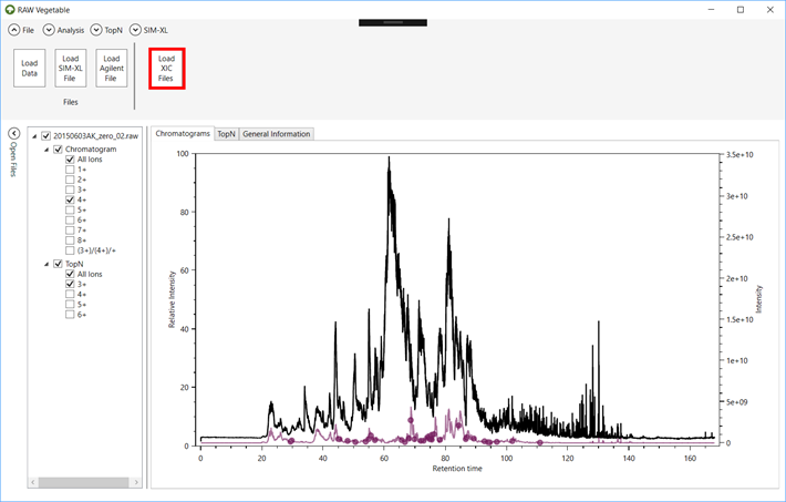
RawVegetable works by loading mass spectrometry data, such as Thermo RAW files, *.mzML, *.ms1 or Agilent files as input. After the spectra has been loaded, the chromatographic profile is displayed and all files loaded are listed on the left side, where the user can choose which ones to view (Figure 1). Once the data has been loaded, there are a few analyses the user can make, such as a charged chromatogram, a TopN distribution, and a search for XL artefacts. Loading PatternLab for proteomics [1] *.xic and *.plp or SIM-XL [2] output files enables a reproducibility analysis. All these features are better described in the following sections.

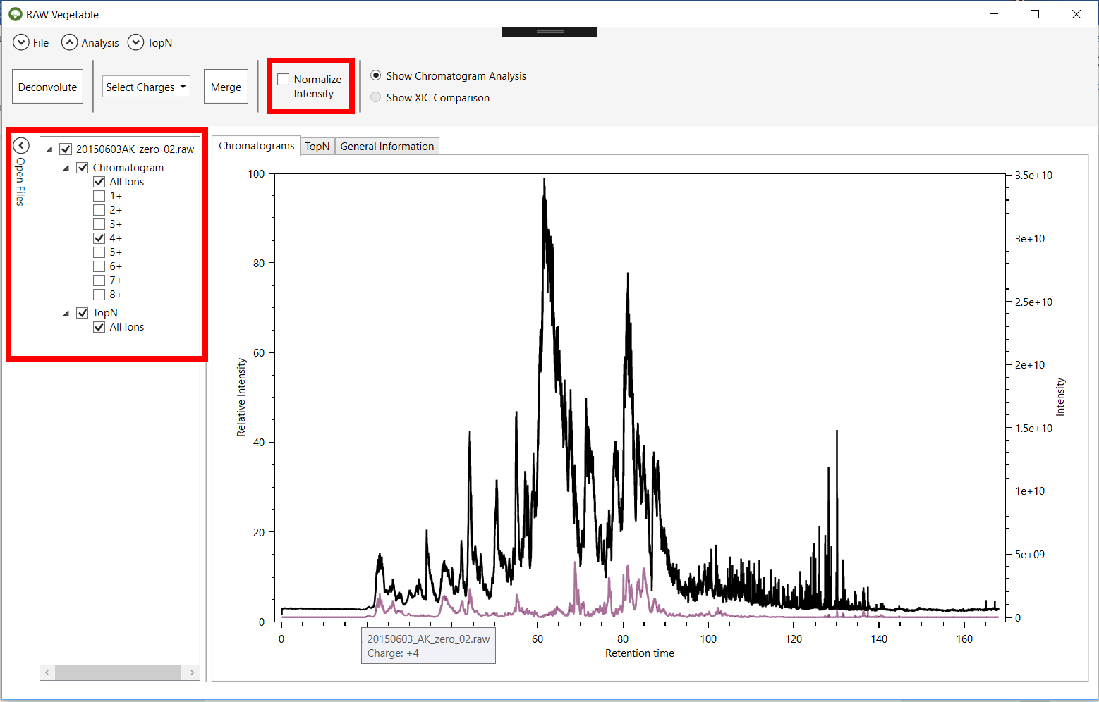
Figure 1 - RawVegetable’s screen after the spectra file have been loaded. On the left side it is possible to see the menu where the user can check which files they wish to view on the screen.

Another analysis the user can make once the spectra files have been loaded is a preliminary search for contaminants. This is based on a list of contaminants described by Keller et al [3], which lists around 700 common contaminants found in mass spectrometry experiments, both with ESI and MALDI ion sources; this list also has a description of the contaminants and the peaks for which to look in mass spectra. The search RawVegetable performs takes all MS1 spectra in a file and looks for all the peaks listed as contaminants for ESI experiments. This can take a few minutes depending on the number of MS1 spectra in the file and results in a table of contaminants and the percentages of spectra they were found in (Figure 2). This search can give an idea of possible contaminants and what to look for in a deeper analysis.

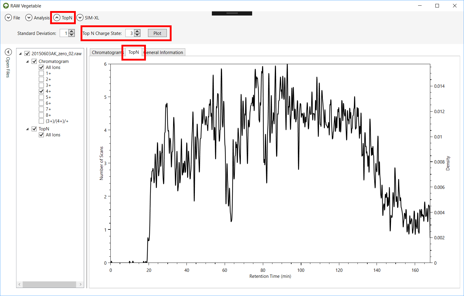
Figure 2 - Resulting table from the preliminary contaminant search showing possible molecules that had their respective peaks flagged in more than 50% of the MS1 scans.

Tables with general statistics such as number of MS and MS/MS spectra, duty cycle average time and chromatography total time and histograms showing the distribution of precursors’ m/z are also available.

1. Charged Chromatogram

Cross-linked peptides will mostly present higher charge states than the linear peptides found in traditional proteomic experiments, due to the existence of a second tryptic peptide in the molecule [7]. Moreover, cross-linked peptides are typically less abundant than linear ones, making optimization imperative. As such, chromatographic optimizations with existing tools are severely limited in the face of XL-MS experiments as their viewers cannot independently account for highly charged peptide ions.

This charge state chromatogram module is tailored towards optimizing chromatography for highly charged ion species by independently plotting the chromatographic profile for each charge state.

In order to do this, all MS1 spectra from each file loaded are deconvoluted using the YADA algorithm [4]. Deconvolution algorithms consist of simplifying a spectrum by merging all isotopic and charge envelopes of a molecule into a single peak.

Isotopic envelopes occur because organic molecules are composed mainly by carbon, which is present in nature with a mass of 13Da instead of 12Da 1% of times. Since cross-linked peptides can contain many carbons, the chance of some of them being ¹³C is quite high. This ends up creating various peaks of the same molecule with the mass difference of a neutron between them, as shown in Figure 3. The fact that this mass difference is known is what allows isotopic envelopes to be used for the determination of the charge of the species represented there, using the following equation:

Here, Peak 1 and Peak 2 are the m/z values of two consecutive peaks in an isotopic envelope (Figure 3) and the neutron mass is around 1Da.

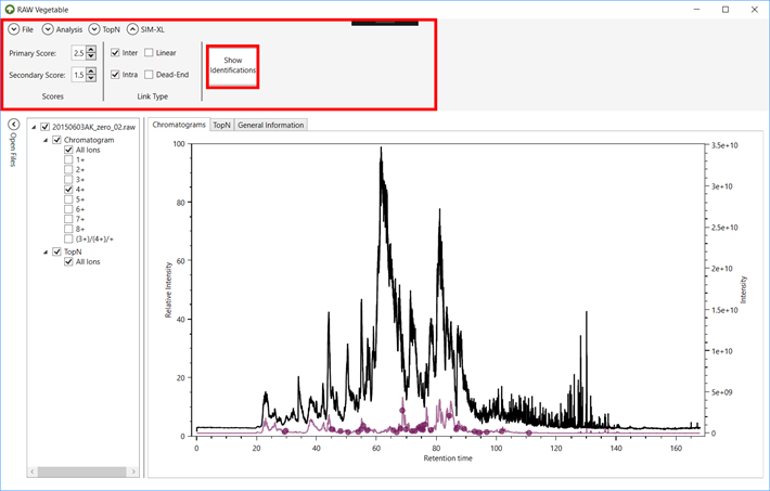
Figure 3 - Representation of an isotopic envelope of a molecule with a lot of carbon atoms. Using equation (1), we discover that the charge of this molecule is 1+, so its mass ranges from 700Da to 712Da, depending on the number of ¹³C it has. In this case, most molecules have six ¹³C, as the most intense peak is the with is the one that has a difference of around 6Da from the first peak.

This algorithm results in a list of all envelopes found in each spectrum, which contains their respective charge and the summed intensities of all peaks in the envelope. With this information, it is possible to choose a single charge and build a chromatogram using the intensities of all envelopes with the selected charge, as shown in Figure 4. This new chromatogram can give insights into when most cross-linked peptides are eluting, as they usually appear with charges 3+ and 4+. The chromatography gradient can thus be altered to prioritize such regions, enrich populations of desired charge states, which could help in the acquisition of more MS2 spectrum from cross-linked species in lieu of conventional, linear peptides.

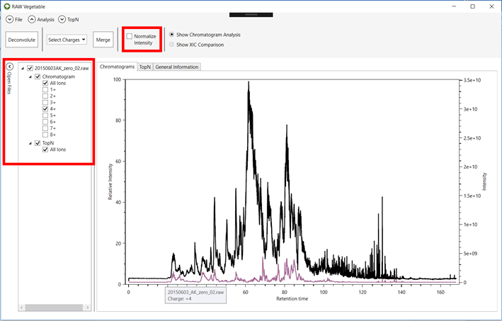
In the GUI, the user can then choose which charge chromatogram to view on the left side of the screen, by checking the boxes of each file, as in Figure 4. It is also possible to normalize the chromatograms on the screen in order to see them all as relative intensities and merge charged chromatograms to see them as one, as in Figure 4.

Figure 4 - RawVegetable's screen after the deconvolution algorithm has run. Represented in black is the full chromatogram of the file selected in the menu on the left; in purple is the chromatogram considering only species with charge 3+. On the top menu it is possible to select charges to merge, as well as normalize the intensities of the chromatograms.

If the search for cross-links has already been performed, it is possible to identify the regions where most of them appeared by loading the SIM-XL output file into RawVegetable. This will result in all identifications being represented in the chromatograms as small circles at the retention time where the scan was extracted. The user can filter the identification by link type and by the scores calculated by SIM-XL (Figure 5).

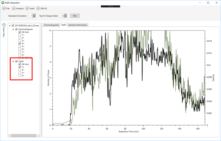
Figure 5 - The software's screen after a SIM-XL output file has been loaded. Here the full chromatogram is represented in black and the charge 4+ is in purple. The purple dots indicate when a cross-link identified with charge 4+ eluted. It is possible to change the score and link type filtering in the top menu.

2. TopN Distribution

This module shows the density estimation of MS2 scans per duty cycle along the chromatography. This allows pin-pointing retention time intervals that could lead to over- or under-sampling, so the necessary gradient adjustments can be done.

In order to do this, the algorithm applies Kernel Density Estimation (KDE) using a Gaussian distribution as the kernel function. Essentially what the algorithm will do is assign a Gaussian for each duty cycle, which will then be multiplied by the number of MS2 scans in that cycle. This will result in several Gaussians overlapping, which will then be summed, generating a density estimation plot, as in Figure 6. This way, every gaussian influences all nearby points in the resulting plot, even if minimally.

Given a dataset composed of the retention time of all MS1 scans, that is, the initial retention time of all duty cycles, as the values of x in a plot, the KDE function used to find their respective y value to generate the density estimation plot is the following [5,6]:

Where n is the number of duty cycles (which is the same as the number of MS1 scans); h is a smoothing factor called bandwidth; is the kernel function, where x is the retention time of the current point in the KDE being calculated and x_i is the x values of the rest of the dataset, that is, the retention time of other duty cycles. The kernel function with x-x_i as parameter represents the influence of all gaussians in the determination of that specific point being calculated, as it returns the intensities of overlapping regions (Figure 6) to be summed, as represented by the summation (∑) which goes from the first retention time (i = 1) to the last (i = n).

Figure 6 - Graphical representation of how the Kernel Density Estimation works. For each duty cycle (DC1, DC2 and DC3) a standard normal distribution is built and then multiplied by its respective number of MS2 scans, generating all these different gaussian with overlapping regions, which will then be summed to create a density estimation plot, such as the represented in orange.

The bandwidth (h) is a smoothing factor which greatly influences the resulting plot and should be as small as possible without causing the plot to be oversmoothed. It can be a tricky parameter to calculate, but for a Gaussian kernel the following equation can be used [7]:

Where σ is the standard deviation of the distribution, which is user-defined, but has a default value of 1; n is the total number of duty cycles.

The kernel function (K(x)) used is a normal (Gaussian) distribution with a mean value of 0, which is defined by the following general form [8]:

Where x is as defined by the KDE equation and σ² is the variance, which is the square of the standard deviation, and has the same value as in the h formula.

The KDE function can then be represented by the following equation:

Applying this function for all duty cycle retention times results in a plot such as the one shown in Figure 7. This plot permits optimizing the chromatography gradient so that the TopN (MS2 scans in a duty cycle) distribution is as wide and homogeneous as possible through time. This optimization can also help shortening the extremities of the chromatography run, thus shortening the time of the experiment.

Figure 7 - RawVegetable's screen after the TopN distribution has been calculated, with the user being able to choose the standard deviation to be used during the calculation. In this case the maximum number of scans in a duty cycle was six spectra and that the equipment did not maintain efficiency throughout the run.

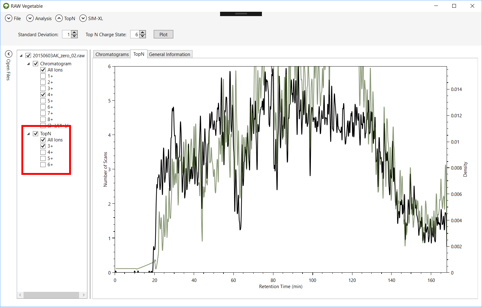
It is also possible to calculate a KDE using only MS2 scans with precursors of a specific charge (Figure 8), to have a better notion of where heavily charged species elute more frequently, similar to the charged chromatograms.

Figure 8 - TopN distribution with specific charge state selection. It is possible to view the TopN distribution of species with a single selected charge, as shown by the green curve, which represents the distribution for charge 3+ precursors; in black is the total TopN distribution.

For experiments where the TopN number has not been set and instead only the time for the duty cycle has been specified in the equipment, it is interesting to look at the performance of the run by viewing the TopN distribution as a frequency plot (Figure 9 (A)). Zooming in regions of interest shows exactly how many scans were obtained in specific duty cycles (Figure 9 (B)). It is also possible to compare the density estimation with the frequency plot by checking both on the menu on the left side of the screen.

Figure 9 - (A) Frequency plot of the MS2 scans during the experiment. (B) Zooming in shows that this plot computes absolute values for the number of scans instead of a distribution as was the case before.

Another application becomes handy especially when using very high-scan rate instruments such as a Thermo Lumos or HFX. The user might set a TopN and get a very homogeneous distribution throughout the run. This could mean that the equipment is being very efficient and even slightly saturated, meaning that the acquisition method could be modified to acquire more MS2 scans per duty cycle, and so take full advantage of the equipment.

3. XL-Artefact

Recently, Giese et al. [9] described the presence of some high scoring identifications wrongly taken for interlink peptides owing to the non-covalent dimerization of a linear peptide and an intralinked one during the ionization step of the mass spectrometry, when the molecules are going to the gas phase. Based on this, we added a feature which flags possible species such as these, which we called XL-Artefacts.

RawVegetable uses a SIM-XL output file to identify whether an artefact is at hand by verifying if XICs of all possible separate species (linear α-peptide and intralinked β-peptide and the inverse) are found during the same retention time range with charges 2+ and 3+. A score is then assigned to the possibly wrong inter-linked XL. This score is calculated as follows: if a linear α-peptide and an intralinked β-peptide or an intralinked α-peptide and a linear β-peptide of any charges have their XICs extracted successfully, one point plus a bonus based on the relative intensities of the XICs are summed to the score. If all four species have valid XICs, then an extra bonus is given. Based on this scoring system, cross-links with scores higher than 1 should already be looked at more closely, however tests made with proteins of known crystallographic structure showed that species with scores higher than 2.5 are the ones more prone to be artefacts.

The result of this algorithm is a table with all interlinked peptides found, with their respective XL-Artefact score and SIM-XL scores listed. The user can also view these possible artefacts represented in the charged chromatograms as red dots, as shown in Figure 10.

Figure 10 - A charge 3+ (in green) and charge 4+ (in blue) chromatograms. The green and blue dots indicate where cross-linked species were identified with charges 3+ and 4+, respectively; the red dots indicate possible XL-artefacts that should be closely analysed.

We exemplify the usefulness of our artefact score on the XL K499-S709 for the HSP90 protein as per one of our experiments. In our example, the XL XIC curve is shown in yellow (Figure 11). The crosslink information is not in agreement with an open conformation model of the HSP90; the Euclidean distance between K499-S709 is of 26Å, while the maximum distance for the DSS crosslinker is of 17Å. The error becomes even higher when comparing this crosslink’s distance constraint result with the closed conformations models of HSP90, which goes up to 56Å. These results corroborate with a wrong identification, due to an artefact of non-covalent association in gas phase. Our “XL-Artefact Analysis” flags this event as it detects the XICs of other possible species. Figure 12 shows in brown and pink the curves for the XICs of the alpha sequence as linear peptide with charges 3+ and 2+; in lilac and green the curves for the XICs of the beta sequence as an intralinked peptide with charges 3+ and 2+; and in yellow, the curve for the XIC of the identified interlink. The results demonstrate that all these peptides eluted during the same time as the “identified interlink”; we also note that the separate species present significantly higher intensities, which strongly suggests that the interlink is in fact a linear alpha peptide non-covalently bound to the intralinked beta peptide in the gas phase.

Figure 11 - XIC Curve for cross-link K499-S709 of the HSP90 protein.

Figure 12 - XIC curves for the individual peptides of the cross-link K499-S709 eluting at the same time range as the identified interlink. In brown and pink, the curves for the XICs of the alpha sequence as linear peptide with charges 3+ and 2+; in lilac and green the curves for the XICs of the beta sequence as an intralinked peptide with charges 3+ and 2+; and in yellow, the curve for the XIC of the identified interlink.

4. Reproducibility Analysis

This module performs all pairwise comparisons of XICs between identifications of different runs, which allows a general view of the chromatographic reproducibility for all runs and therefore to quickly locate problematic MS run.

In order to perform this analysis, RawVegetable needs the PatternLab’s *.xic or *.plp result, or the SIM-XL output files as input. The software will then group all common peptides between the files and proceed to compare their XICs (which should already have been calculated and stored in the input files). This comparison between common peptides is made for each pairwise combination of files, with the XICs of one file representing the x values and the XICs of the other file, the y values. With these values in hand, it is possible to calculate a similarity score between the files; the user can choose the following metrics to use for the score: r², k or k².

The r² metric is the coefficient of determination and calculates how well a set of points fits a linear regression; in this case, a line represented by the equation y = x. The general formula for r² is the following [10]:

Where y_i the actual value of y being used; ŷ_i is the predicted value of y_i, following the equation y = x and ӯ is the mean of the y values. In this case, the closer the r² is to 1, the more similar are files being compared.

The k metric is the Euclidean distance between the XIC values of each file. The XIC values of the first file will be represented by the vector x, where x = (x₁, x₂, …, x_n) and the second file by y¸ where y = (y₁, y₂, …, y_n). First the values are normalized to be within a range of 0 to 1 and then the Euclidean distance can be calculated using the following equation [11]:

Using this metric gives an information which is the inverse of r²; the closer the k value is to 0, the more similar are the files.

Another metric that can be used is the square of the k value (k²), which is calculated the same way, but accentuates the similarities between files.

The calculation of these scores produces a heatmap comparing files using the chosen metric. The plots generated using the different score systems are shown in Figure 13.

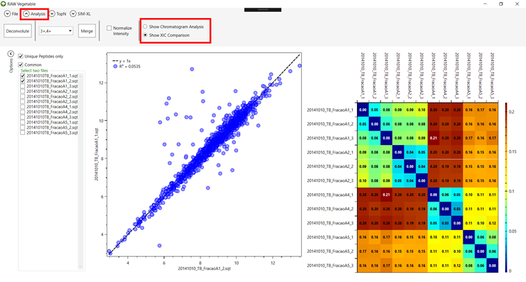
It is also possible compare two specific files by marking them on the left side of the screen. This will result in a dot plot of all common peptides between the files according to their XIC values, along with a trend line and the score value, as in Figure 14.

This analysis allows to easily pinpoint problematic experiments and determine whether a replicate should be used during the research or not.

Figure 13 - The heatmaps generated using k (A), k² (B) and r² (C) as score metrics. It is possible to see that while the colour system changes, the information given is the same, the technical replicates (in groups of three in the order shown) are very similar, while some of the biological replicates are quite different.

Figure 14 - Dot plot comparing the XIC of common peptides of two different files, with the score shown in the left as the metric k, and a trendline for the equation y = x.

5. Precursor ion dissociation efficiency

In this feature, the proportion between the intensity of the precursor peak in a MS2 scan and the total intensity of all peaks in the same scan is calculated. The motivation is to assess how much of the MS2 scan is composed of the precursor and thus evaluate the collisional energy and dissociation process efficiency. In brief, the software does this process for every MS2 scan to ultimately present the results as histogram (Figure 15). The higher the distribution’s density is found near zero, the more efficient the fragmentation is, as the precursor peak is responsible for less of the total ion current of the scan.

Figure 15 - Histogram of the ratios between precursor intensity and total ion current of a MS2 scan, which can give some information on the fragmentation efficiency of an acquisition. The different colours represent different experiments being compared in the same plot.

References:

[1] P.C. Carvalho, D.B. Lima, F.V. Leprevost, M.D.M. Santos, J.S.G. Fischer, P.F. Aquino, J.J. Moresco, J.R. Yates, V.C. Barbosa, Integrated analysis of shotgun proteomic data with PatternLab for proteomics 4.0, Nat. Protoc. 11 (2015) 102–117. https://doi.org/10.1038/nprot.2015.133.

[2] D.B. Lima, J.T. Melchior, J. Morris, V.C. Barbosa, J. Chamot-Rooke, M. Fioramonte, T.A.C.B. Souza, J.S.G. Fischer, F.C. Gozzo, P.C. Carvalho, W.S. Davidson, Characterization of homodimer interfaces with cross-linking mass spectrometry and isotopically labeled proteins, Nat. Protoc. 13 (2018) 431–458. https://doi.org/10.1038/nprot.2017.113.

[3] B.O. Keller, J. Sui, A.B. Young, R.M. Whittal, Interferences and contaminants encountered in modern mass spectrometry, Anal. Chim. Acta. 627 (2008) 71–81. https://doi.org/10.1016/j.aca.2008.04.043.

[4] P.C. Carvalho, T. Xu, X. Han, D. Cociorva, V.C. Barbosa, J.R. Yates, YADA: a tool for taking the most out of high-resolution spectra, Bioinformatics. 25 (2009) 2734–2736. https://doi.org/10.1093/bioinformatics/btp489.

[5] M. Rosenblatt, Remarks on Some Nonparametric Estimates of a Density Function, Ann. Math. Stat. 27 (1956) 832–837. https://doi.org/10.1214/aoms/1177728190.

[6] E. Parzen, On Estimation of a Probability Density Function and Mode, Ann. Math. Stat. 33 (1962) 1065–1076. https://doi.org/10.1214/aoms/1177704472.

[7] B.W. Silverman, Density estimation for statistics and data analysis, Chapman & Hall/CRC, Boca Raton, 1998.

[8] J.K. Patel, C.B. Read, Handbook of the normal distribution, 2nd ed., rev.expanded, Marcel Dekker, New York, 1996.

[9] S.H. Giese, A. Belsom, L. Sinn, L. Fischer, J. Rappsilber, Noncovalently Associated Peptides Observed during Liquid Chromatography-Mass Spectrometry and Their Effect on Cross-Link Analyses, Anal. Chem. 91 (2019) 2678–2685. https://doi.org/10.1021/acs.analchem.8b04037.

[10] T.O. Kvalseth, Cautionary Note about R 2, Am. Stat. 39 (1985) 279. https://doi.org/10.2307/2683704.

[11] H. Anton, Elementary linear algebra, 7th ed, John Wiley, New York, 1994.