RawVegetable’s Tutorial

PROTOCOL

RawVegetable requires Thermo mass spectrometer RAW files, *.mzML or Agilent files for the main feature to function. The chromatography reproducibility feature requires PatternLab for proteomics’ *.xic or *.plp files or a SIM-XL output file. In order to view identifications along the chromatogram, a SIM-XL file is required.

Example dataset can be downloaded here.

Extended information on how the modules work can be found here.

HOW TO USE

1. Installing RawVegetable

The latest version of the RawVegetable software is available here. The software requires version 4.7.2 or higher of the .NET framework, which can be downloaded here, if it is not already installed.

For reading Thermo RAW files, the MSFileReader must be installed. Download it by creating an account at Thermo®, then logging and choosing Utility Software.

2. Charge State Chromatogram

2.1. Select the chosen RAW or mzML files by clicking on the “Load Data” button (which can be found in the “Files” menu). To open an Agilent file, click on “Load Agilent File” (Figure 1). You can also simply drop the files you wish to analyze.

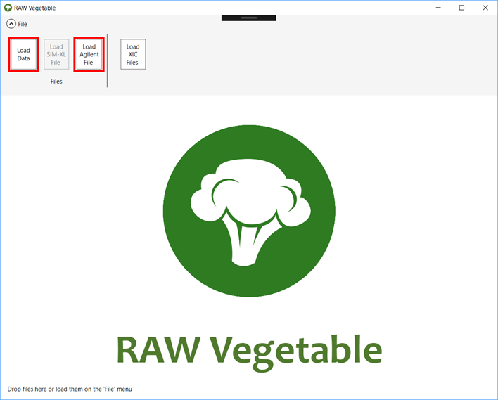
Figure 1 - Starting RawVegetable Screen.

2.2. First you will have to choose between extracting the chromatogram as Total Ion Current (TIC) or Base Peak Only, as shown in Figure 2.

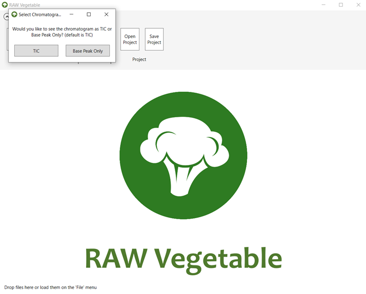
Figure 2.

2.3. After the file loads, the screen will be as shown in Figure 3. Information such as the number of MS1 and MS2 scans can be seen on the “General Information” tab.

2.4. To see all the files loaded and choose which ones to show on the viewer, click on the “Open Files” menu (Figures 3 and 4). Simply click on the checkbox to view/hide a chromatogram.

2.5. In order to see the charge-specific chromatograms, click on the “Deconvolute” button (Figure 3). This process will deconvolute all the files that are checked in the “Open Files” menu (Figure 4) and can take minutes to conclude according to the size of the files.

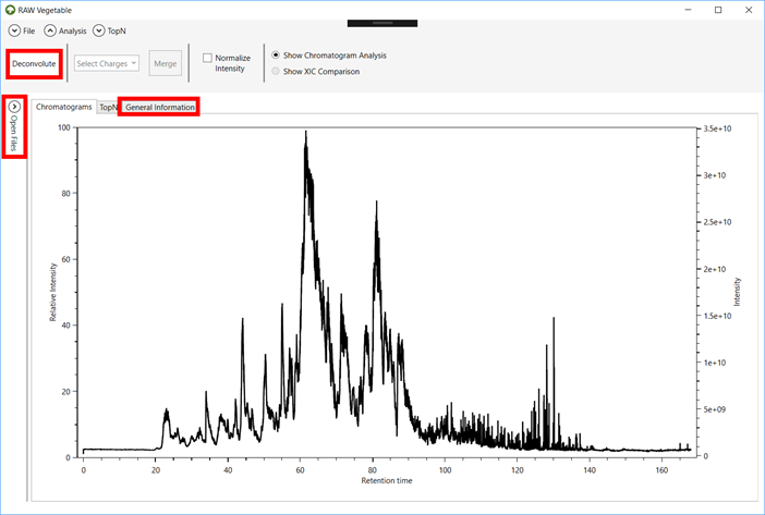
Figure 3.

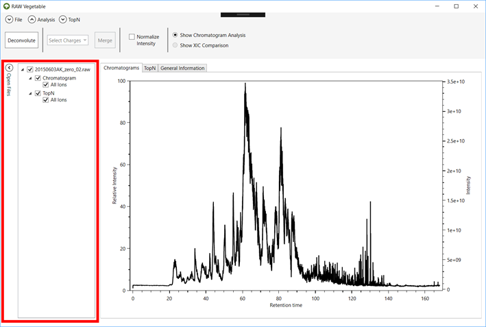
Figure 4.

2.6. Once the deconvolution is complete, select the charge you want to view on the “Open Files” menu (Figure 5). You can identify the chromatograms by hovering the mouse on top of it.

2.7. To see all chromatograms as relative intensities (normalized values), click on the “Normalize Intensity” checkbox (Figure 5).

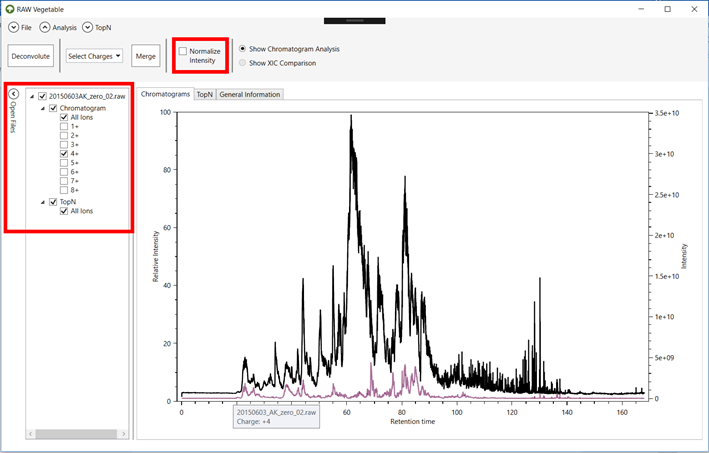
Figure 5.

2.8. If you want to see more than one charge as a single chromatogram, select the charges on the combo box shown in Figure 6 and click the “Merge” Button. The merged chromatogram will now be shown on the “Open Files” menu.

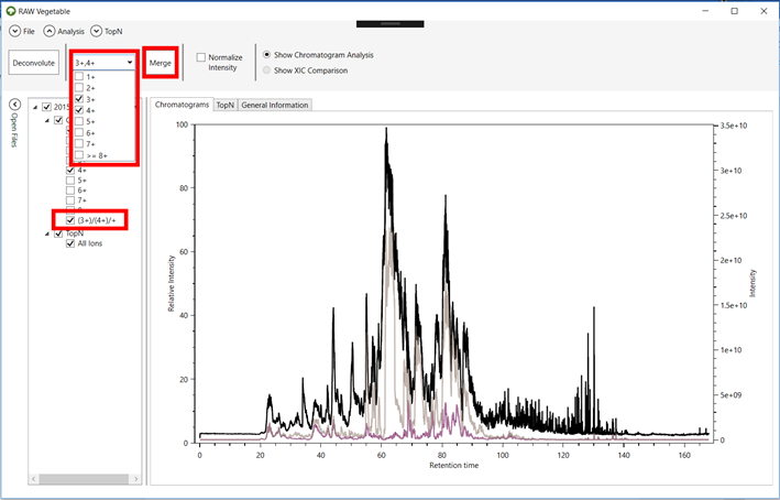
Figure 6.

2.9. If you have a SIM-XL output file and wish to see where the cross-links were identified, click on the “File” menu and on the “Load SIM-XL File” button (Figure 7).

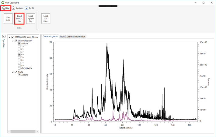
Figure 7.

2.10. After the file loads, the “SIM-XL” menu will appear on top, where you can filter the identifications by score and link type. To see the cross-links, click on the “Show Identifications” button (Figure 8).

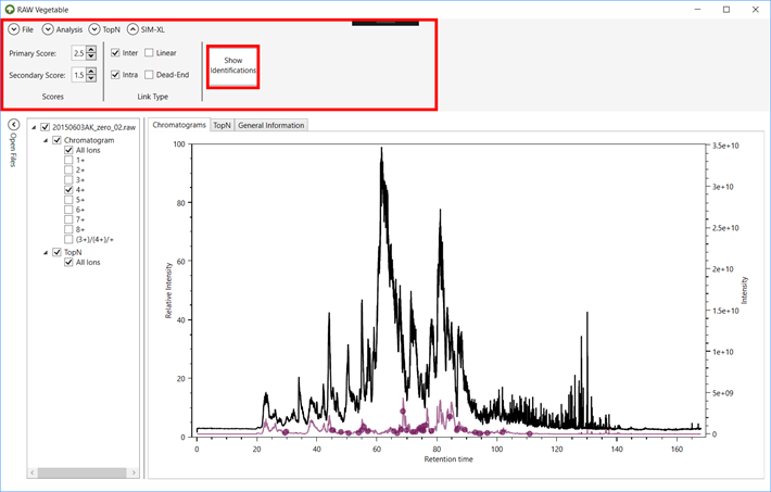
Figure 8.

3. TopN Density Estimation

3.1. To see the TopN density estimation, click on the “TopN” tab after loading the files (Figure 9).

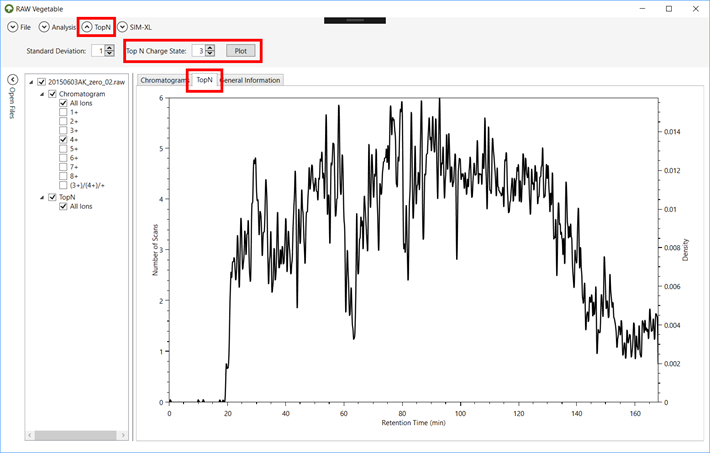
Figure 9.

3.2. To see the density estimation only of precursors of a specific charge, go to the “TopN” menu, select the charge and click on “Plot” (Figure 9). This might take a while according to the number of MS2 scans acquired.

3.3. Once the density estimation has been calculated, the curve will appear on the TopN viewer and you can view/hide it by clicking on the checkbox under the “TopN” item for each file on the “Open Files” menu (Figure 10).

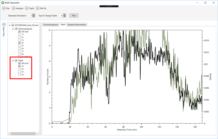
Figure 10.

4. Chromatography reproducibility

4.1. Load either PatternLab for proteomics’ *.xic or *.plp files, or SIM-XL output files (*.simxlr) by going to the “File” menu and clicking on “Load XIC Files” (Figure 11).

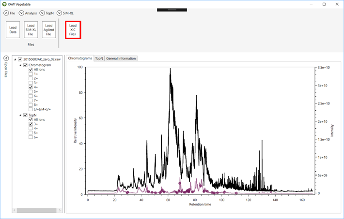
Figure 11.

4.2. You can see the heatmap generated by the comparison of all files on the right, or you can choose two files to compare on the left side (Figure 12). It is also possible to choose to look for all peptides instead of unique or common ones, by clicking on the checkboxes on the left.

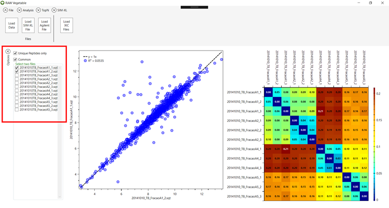
Figure 12.

4.3. To go back to seeing the chromatography analysis, go to the “Analysis” menu and click on the “Show Chromatogram Analysis” checkbox (Figure 13).

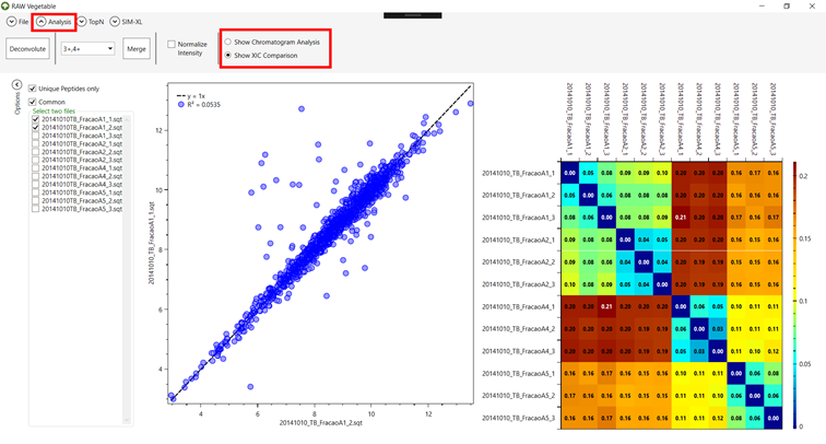
Figure 13.