DiagnoTop describes a method based on spectral clustering and pattern recognition to statistically list discriminant spectral clusters based on MS/MS data obtained from the fragmentation of intact proteins, without database search. Our approach uses Top-Down Garbage Collector (TDGC) to serve as a gatekeeper and only allow high-quality spectra feed to DiagnoProt, a software previously introduced by us, that shortlists discriminative spectral clusters.

This tutorial describes all the necessary steps for using and understanding our computational approach. The installation section shows how to install and configure the software. The how it works section details the theory and methods employed. We strongly recommend its reading before any attempt to use the software, as it will provide an understanding of what is going on behind the scenes so that the parameters can be properly set according to the experimental setup at hand. Finally, the how to use it section shows where one can click to get things done.

If there are still questions after reading this tutorial, a Forum is made available for further assistance.

Overview

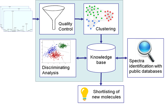Figure 1 DiagnoTop workflow.

The general workflow of DiagnoTop is summarized in Figure 1. The first step is to use the quality control filter (TDGC) on all MS/MS spectra to select the high-quality ones. TDGC uses an automatic scoring function to classify whether a mass spectrum is noisy or not. The software only considered noisy spectra if at least 20 isotopic envelopes could be identified by Y.A.D.A.; for spectra with a good signal to noise ratio, only 5 isotopic envelopes were required. Isotopic envelopes with a 1+ profile were not considered. In addition, the algorithm examined features within the 500 – 1500 m/z range. At the end of this first step, TDGC also helps to speed up the processing and increase clustering precision. In what followed, DiagnoTop is used to generate the Knowledge Base (KB). We define KB as a collection of spectral clusters derived from the various biological conditions (in this case, bacterial strains). We define a spectral cluster as a set of similar MS/MS spectra grouped according to a similarity function, in our case, the spectral angle. This aims to group all similar MS/MS spectra arising from the fragmentation of the same proteoform. The second part of DiagnoTop includes a comparison of all the spectral clusters that have been previously created. The Jaccard index was used to determine the similarity between different spectral clusters by comparing all similar MS/MS spectra originating from the different biological conditions. At the end, DiagnoTop generated as results, a PCA and a heatmap in order to allow several kinds of analyses.

---

Binning

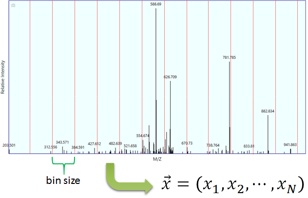Figure 2 Example of a binned spectra.

Binning is an operation that transforms a spectrum into a vector (Figure 2). The objective of binning is to make a summary of the spectrum and to optimize mathematical calculations. A bin is by definition an interval [l,u) of m/z values. The bin’s lower (l) and upper (u) bounds are represented as red lines in Figure 2. The binning procedure is controlled by the parameters in Table 2.

Table 2 Binning parameters.

Parameter	Default Value
Bin Offset	0.0
Bin Size	0.02
Min. Bin m/z	200
Max. Bin m/z	1700

The binning procedure works as follows. All peaks whose m/z are bellow Min. Bin m/z or above Max. Bin m/z are discarded. Let o be the value of Bin Offset and s the value of Bin Size. A number of bins is then created, the first one being [o, o+s), the second [o+s,o+2s), and the ith one for i > 0 being [o+(i-1)s, o+is). Of course, the total number of bins will be limited by the binning parameters. When bins are created, all peak intensities inside each bin are summed up and saved in a normalized vector.

---

Clustering

The objective of clustering is to find spectra that are very similar, thus doing away with redundancy in the KB. The clustering algorithm is controlled by the parameters in Table 3. Note that the retention time tolerance (Ret. Time Tolerance) is an optional parameter, and by default it is set to positive infinity.

Table 3 Clustering parameters.

Parameter	Default Value
Similarity Threshold	0.4
Precursor Tolerance	3.5
Ret. Time Tolerance	10

Two spectra are said to be similar to each other if, and only if, the difference in their precursors’ m/z is within Precursor Tolerance, the difference in their chromatography retention times is within Ret. Time Tolerance, and the similarity function between them is above the Similarity Threshold. DiagnoTop finds all similar spectra, cluster them and stores them at the KB.

---

Discriminating analysis

A discriminative analysis requires a KB with at least 2 conditions. By comparing the collections of clusters, the algorithm finds all discriminating clusters for each biological condition in the KB taking into account spectral similarities and quantitative data.

If a proteomic search such as peptide spectrum matching (PSM) is performed on these clusters, it is expected that many of them will remain unidentified. In order to find these “gold”, high-quality unidentified spectra, you must run a proteomic search on your KB and set a maximum XCorr score. The default Max. XCorr is 1.5, which is a very low value, so a score bellow this value is usually considered a false identification. All discriminating spectra that are bellow Max. XCorr are said to be “gold” spectra because they passed the QC but could not be identified by the proteomic search engine.

---

Spectral profile classifier

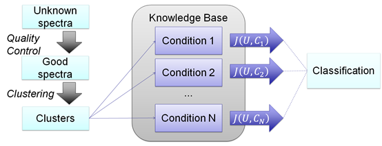Figure 3 Spectral Profile Classifier.

The spectral profile classifier tries to discover the biological condition of an unknown sample by making cluster comparisons between the known conditions in the KB. The spectra of a sample of unknown condition pass through the same QC and clustering procedures used in the KB creation. Then, using a cluster set similarity score, the unknown sample is assigned to the highest ranking condition in the KB.

---

Principal Component Analysis

A Principal Component Analysis (PCA) may be performed on the KB to provide an intuitive view of the biological samples and their relations. The PCA plots the dissimilarities/distances between samples and conditions in a chart. With this procedure, it is possible to have a graphical overview of the samples in the KB. It is expected that biological samples belonging to the same biological condition will share much biological material, and therefore they may be graphically closer in the plot.

Creating a Knowledge Base

Before searching for discriminative spectra or starting the spectral profile classifier, a KB must be generated with at least 2 biological conditions. In what follows, the creation of a KB using DiagnoProt's Knowledge Base Manager is demonstrated.

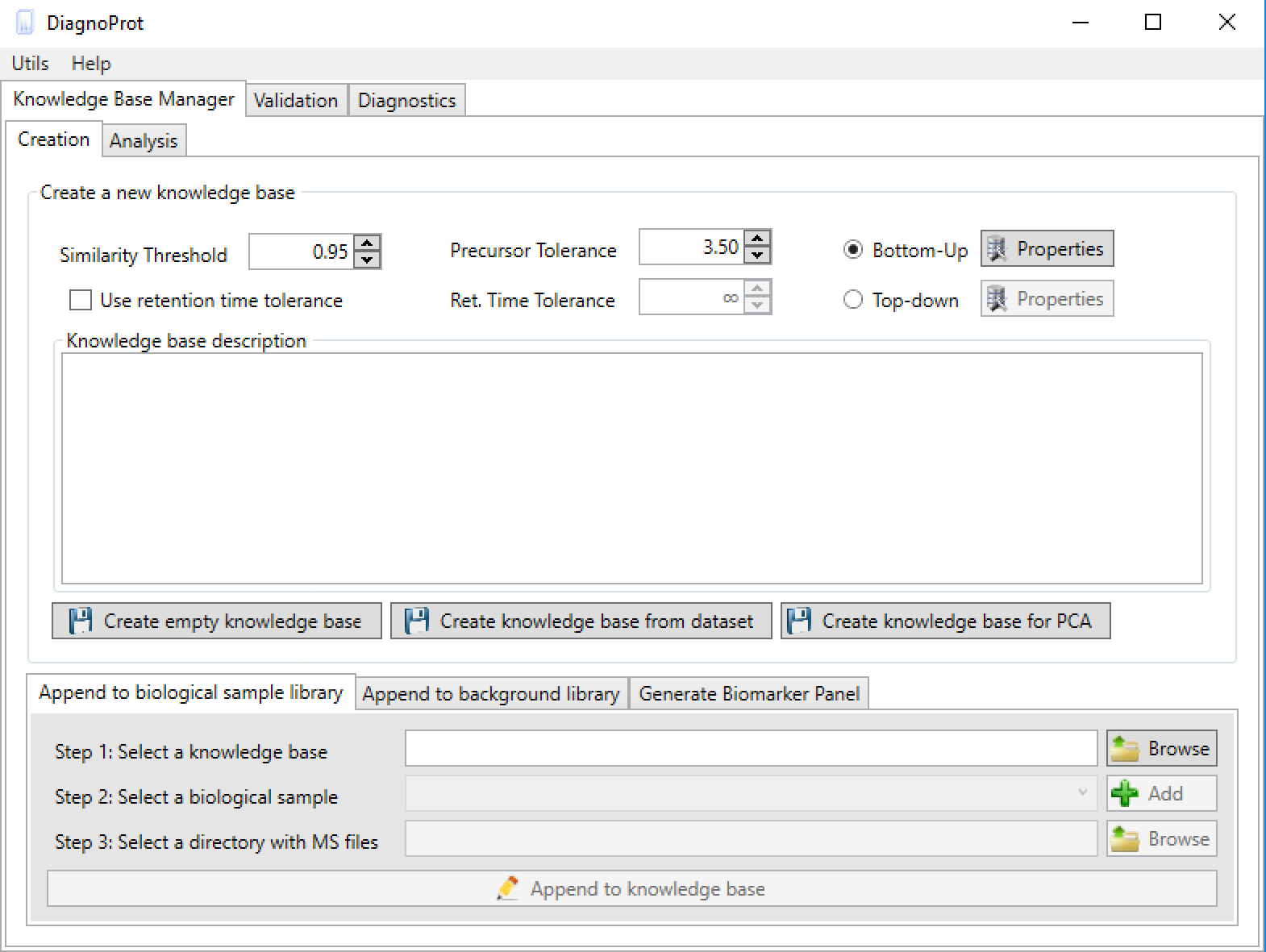Figure 4 KB Manager interface.

As soon as DiagnoProt is launched, the KB Manager interface can be seen (Figure 4). One can either create an empty KB or create a KB automatically from a dataset of MS files.

To create the KB automatically, set the clustering parameters (Similarity Threshold, Precursor Tolerance, and Ret. Time Tolerance), chose a general setup (Bottom-Up, for shotgun proteomics data, or Top-Down*), add a KB description, and click on the button "create a knowledge base from dataset". A dialog box will prompt the user to inform the root directory of the MS files, and that’s it! With just a few clicks of the mouse, the software will start computing clusters and will create a KB automatically. Needless to say, the MS files must be supported by the software. Currently, DiagnoProt supports the RAW (Thermo Fischer Scientific®) and MS2 file formats, but other formats will be supported shortly. The fungi dataset, described in our paper, is available for download. In addition, for the "KB with one click" option to work, the MS files must be organized in a logical structure enabling DiagnoProt to determine the biological conditions linked to each file. An example of a valid directory structure is shown in Figure 5. Fungi_Dataset is the dataset's root directory. Bellow the root directory, the directories of each biological conditions are found. In turn, under each biological condition directory, directories with biological replicates, containing their respective MS, are found. In this way, just by parsing the directory structure, DiagnoProt will take all MS files in the Aoryzae1 directory to belong to one biological sample of Aspergillus oryzae.

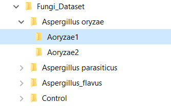Figure 5 MS files directory structure for automatic KB creation.

Besides creating a KB from a dataset of MS files, one can also create an empty KB from scratch by clicking on the button “create empty knowledge base”. In either way, one will end up with a .PKB file that stores the KB.

---

Appending new data into a Knowledge Base

Once a *.pkb file is created, one can add new biological conditions to the KB and new spectra to an existing condition. In the "KB Manager > Creation > Append to biological sample" tab, select the KB file you wish to update, select an existing biological condition or add a new one by clicking the "add" button, and chose a directory with MS files. All the spectra in the MS files will be clustered and merged with the spectra already saved in the KB.

---

Shortlisting discriminative spectra

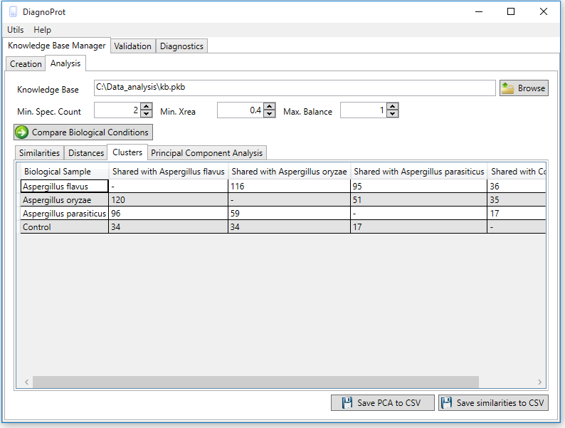Figure 6 KB Manager Analysis interface.

The discriminating analysis is done using the KB Manager Analysis interface (Figure 6). One must input the KB file, set the QC parameters: Min. Spec. Count, Min. Xrea and Max. Balance, and click on the "compare biological conditions" button. When the computations are complete, all clusters that occur in other conditions and the unique clusters of each condition will be shown in the clusters tab. Each cell in the clusters table shows the number of spectra in the intersection, and the last column shows the number of unique spectra.

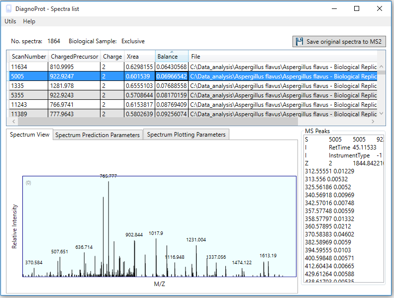Figure 7 Spectrum Viewer explorer.

If one double-clicks on any cell of the clusters table, the Spectrum Viewer explorer will pop up listing all the spectra linked to that cell (Figure 7). Here, one can view the spectrum and other relevant information, such as precursor m/z, precursor charge, Xrea, and Balance score. This interface also enables saving the original spectra to the MS2 format for further analysis by a search engine.

---

Finding gold spectra

To find "gold spectra", that is, high-quality discriminative spectra that remain unidentified by a search engine, DiagnoProt recognizes the SQT formats generated by search engines like Comet [2] (embedded in PatternLab [3]), SEQUEST, or ProLuCID. To evaluate the spectra, save the exclusive clusters to MS2 file format using the Spectral Viewer explorer (Figure 7), run the search on these MS2 files, and then open the Find Gold Spectra using the utilities menu of DiagnoProt (Figure 8).

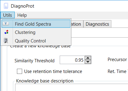Figure 8 Find Gold Spectra on Utils menu item.

In the Find Gold Specra interface (Figure 9), inform the MS2 file that was saved, the SQT file(s), and the KB file. Then set the QC parameters and a maximum XCorr for spectra to be considered unidentified. The default value for Max. XCorr is 1.5, which is a very low cross-correlation score and is usually not considered a match. Click on the save button, and when the search is finished, DiagnoProt will show all high-quality spectra that were not identified by the PSM search engine in the Spectrum Viewer explorer (Figure 7).

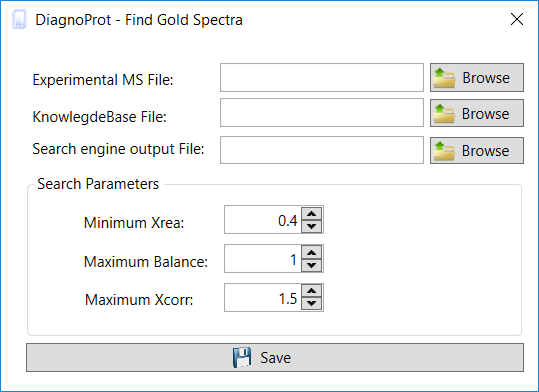Figure 9 Find Gold Spectra interface.

---

Spectral Profile Classifier

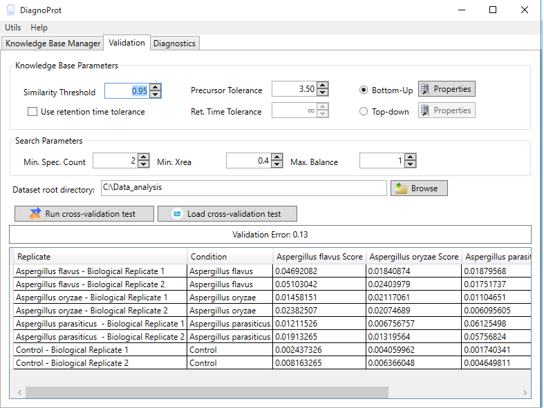Figure 10 Spectral Profile Classifier validation interface.

The Spectral Profile Classifier's performance can be validated on your KB. DiagnoProt's validation tab (Figure 10) runs a leave-one-out cross-validation (LOOCV) test on your data and gives you an estimate of the classification error outside your sample dataset. This test works by temporarily removing all the clusters from a biological sample from the KB, treating it as a unknown sample, and then submitting it to the classifier. After repeating the procedure for all biological samples, a validation error estimate will be shown as well as the classifier’s assignment to each replicate. To run the test, you must set the clustering parameters, the QC parameters, and the dataset root directory. Your MS files in the root directory must follow the same directory structure previously described for creating a KB with a single click.

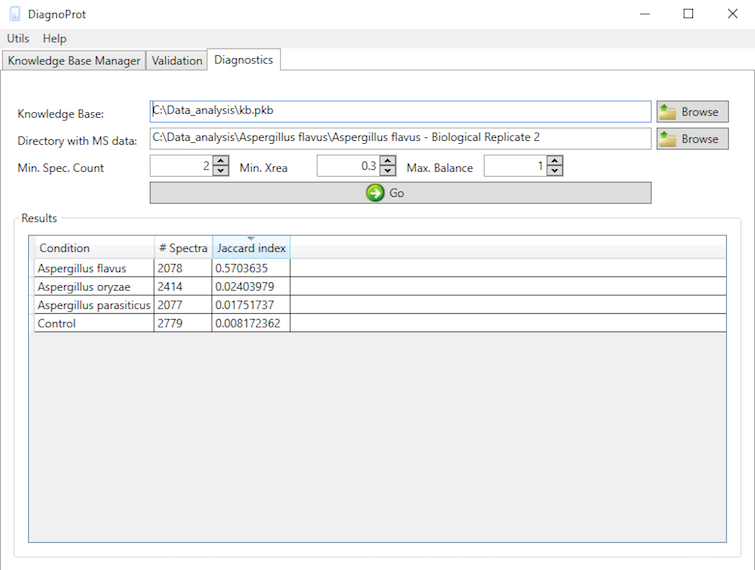Figure 11 Diagnostics tab.

If you're satisfied with the validation results, you can apply the classifier and your KB data in the classification of unknown conditions. This is done in the Diagnostics tab (Figure 11). This tool performs a spectral cluster profile classification of unknown samples using Jaccard index comparisons between all the conditions in the KB and the unknown sample. To run the diagnostics, chose a KB, chose a directory with MS files from the unknown condition, set QC parameters, and click on the "GO" button. When all computations are done, the Jaccard indexes between the unknown sample and all conditions will be shown in the table.

---

PCA plot

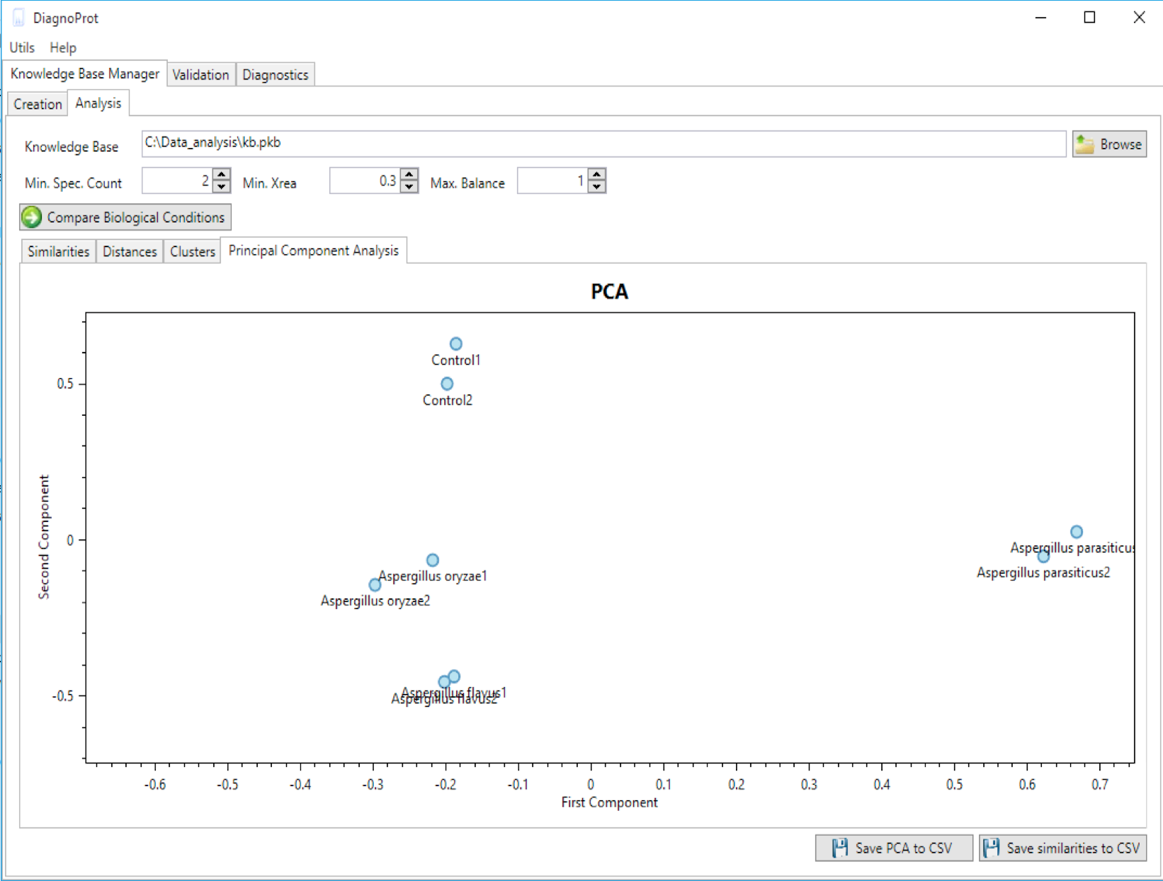Figure 12 PCA plot of biological samples tool.

DiagnoProt can generate a PCA plot showing how biological samples are close to one another (Figure 12). To do this, chose a KB, set QC parameters, and click on the "compare biological conditions" button. DiagnoProt will compute Jaccard indexes between all pairs of biological samples, perform a projection on the direction of greatest data variance, and plot each sample in a two-dimensional chart. Each point in the chart represents a biological condition. It is expected that samples from the same condition will appear close to one another in the PCA plot.

---

Limitations

The spectral library should be generated only with files originating from the mass spectrometry protocol. At this point, we do not recommend clustering spectra from different types of equipment.

1. S. Na and E. Paek, "Quality Assessment of Tandem Mass Spectra Based on Cumulative Intensity Normalization", Journal of Proteome Research, vol. 5, no. 12, pp. 3241-3248, 2006.
2. Paulo C Carvalho 1, Tao Xu, Xuemei Han, Daniel Cociorva, Valmir C Barbosa, John R Yates 3rd, "YADA: a tool for taking the most out of high-resolution spectra", 2009.
3. Eng, M. Hoopmann, T. Jahan, J. Egertson, W. Noble and M. MacCoss, "A Deeper Look into Comet—Implementation and Features", Journal of The American Society for Mass Spectrometry, vol. 26, no. 11, pp. 1865-1874, 2015.
4. P. Carvalho, D. Lima, F. Leprevost, M. Santos, J. Fischer, P. Aquino, J. Moresco, J. Yates and V. Barbosa, "Integrated analysis of shotgun proteomic data with PatternLab for proteomics 4.0", 2016.